R-CNN

Goal: Object recognition
Paper: https://arxiv.org/abs/1311.2524

Region proposals

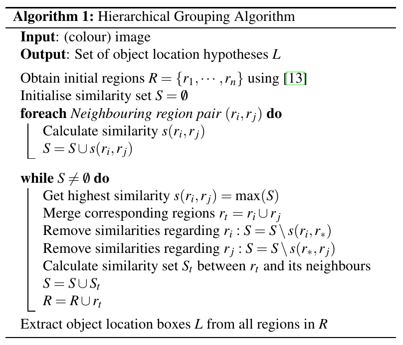
Use selective search to extract 2000 region proposals per image.

Selective search

First use [13] Efficient Graph-Based Image Segmentation to create initial regions. Then calculate the similarties \(s(r_i,r_j)\) between every neighbouring regions. The similarity contains four parts \(s_{color}\), \(s_{texture}\), \(s_{size}\) and \(s_{fill}\), these measures are all in range \([0,1]\).

1. \(s_{color}(r_i,r_j)\) measures color similarity for a regular RGB or HSV image it obtains histograms using 25 bins for each channel \(C_i = {c_i^1,…,c_i^{n}}\) \(n=25\times3\) (The histograms are normalized using L1-norm) and the similarity is measured using histogram intersection \(s_{color}(r_i,r_j)=\sum\limits_{k=1}^{n}min(c_i^k,c_j^k)\).
2. \(s_{texture}(r_i,r_j)\) measures texture similarity, it represents texture using SIFT-like algorithm which takes Gaussian derivatives in eight directions. Then for each channel it extracts a histogram using 10 bins \(T_i = \set{t_i^1,\dots,t_i^{n}}\) \(n=8\times10\times3\) (The histograms are normalized using L1-norm) abd the similarity is measured using histogram intersection \(s_{texture}(r_i,r_j)=\sum\limits_{k=1}^{n}min(t_i^k,t_j^k)\).
3. \(s_{size}(r_i, r_j)\) in order to prevent a single region keeps merging other regions, this algorithm obtains a button up approach to encourage small regions to merge early \(s_{size}(r_i,r_j)=1-\dfrac{size(r_i)+size(r_j)}{size(im)}\), \(size(r)\) gives the size of region \(r\) in pixels.
4. \(s_{fill}(r_i,r_j)\) measures how well two regions fit into each other in order to fill gaps and avoid any holes in merging process. Define \(BB_{ij}\) to be a bounding box around \(r_i\) and \(r_j\). \(s_{fill}(r_i,r_j)=1-\dfrac{size(BB_{ij})-size(r_i)-size(r_j)}{size(im)}\)

The final similarity is the combination of the four measures where \(a_i\) is either \(0\) or \(1\).
$$
s(r_i,r_j)=a_1s_{color}(r_i,r_j)+a_2s_{texture}(r_i,r_j)+a_3s_{size}(r_i,r_j)+a_4s_{fill}(r_i,r_j)
$$

Feature extraction

First, the arbitrary-shaped regions are warped to the required size. Then the extraction step is done by foward a mean-substracted 227x227 RGB image through AlexNet which is pre-trained on ImageNet dataset.

Here might be confusing as the original paper ImageNet Classification with Deep Convolutional Neural Networks states that the size of input image is 224x224. According to this discussion this is a mistake, the layer size will only make sense if the input size is 227x227. Moreover, Caffe framework, whick is used in this paper, expects the same input size as well.

Classify regions

After extracting feature vector for every region proposals, each feature vector is then scored by the SVM trained for each class.

Bounding box regression

Predict a new bounding box for the detection using a class-specific bounding box regressor as the bounding box extracted by selective search might have a relative low IoU. By adjusting the bounding box closer to ground-truth, we can get a more accurate detection result.

Input of the regressor is a set of training pairs \({(P^i, G^i)}_{i=1,\dots,N}\), where \(P^i=(P_x^i,P_y^i,P_w^i,P_h^i)\) is the proposal bounding box and \(G^i=(G_x^i,G_y^i,G_w^i,G_h^i)\) is the ground-truth bounding box. The goal is to find a transformation that maps \(P\) to \(G\).
$$
\displaylines{
\hat{G}_x=P_wd_x(P)+P_x\\
\hat{G}_y=P_hd_y(P)+P_y\\
\hat{G}_w=P_w\ \text{exp}(d_w(P))\\
\hat{G}_h=P_h\ \text{exp}(d_h(P))
}
$$

\(d_x\), \(d_y\) specify a scale-invarient translation of the center of the bounding box, while \(d_w\), \(d_h\) specify a log-space translation. Transform function is modeled as \(d_\star(P)=\textbf{w}_\star^T\phi_5(P),\ \star \in \set{ x, y, w, h }\) where \(\phi_5(P)\) is the feature vector output by pool5 of the CNN used in feature extraction, \(\textbf{w}_\star\) is a learnable model parameter vector. This paper applies SSE(Error Sum of Squares) loss with L2 regularization.

$$
\displaylines{
\mathcal{L} = \sum_{i}^{N}(t^i_\star-d_\star(P^i))^2+\lambda\lVert{\hat{\textbf{w}}_\star}\rVert^2 \\
\textbf{w}_\star = \underset{\hat{\textbf{w}}_\star}{\text{argmin}}\ \mathcal{L}
}
$$

$$
\displaylines{
t_x = (G_x-P_x)/P_x \\
t_y = (G_y-P_y)/P_y \\
t_w = \text{log}(G_w/P_w) \\
t_h = \text{log}(G_h/P_h)
}
$$